Unit Tests
Comprehensive Unit Tests
There are a few unit tests in Microphysics that operate on a generic
EOS, reaction network, conductivity, or some smaller component to
Microphysics. Many of these tests exercise the main interfaces in
Microphysics/interfaces/ and the code that those call.
These tests compile using the AMReX build system, which assumes that
main is in C++, so each have a main.cpp driver. The files
Microphysics/Make.Microphysics and
Microphysics/Make.Microphysics_extern provide the macros necessary
to build the executable. Runtime parameters are parsed in the same
fashion as in the application codes, using the write_probin.py
script.
Note
Most of these tests work with MPI+OpenMP, MPI+CUDA, and MPI+HIP
EOS test
Microphysics/unit_test/test_eos/ is a unit test for the equations
of state in Microphysics. It sets up a cube of data, with
\(\rho\), \(T\), and \(X_k\) varying along the three
dimensions, and then calls the EOS in each zone. Calls are done to
exercise all modes of calling the EOS, in order:
eos_input_rt: We call the EOS using \(\rho, T\). this is the reference call, and we save the \(h\), \(e\), \(p\), and \(s\) from here to use in subsequent calls.eos_input_rh: We call the EOS using \(\rho, h\), to recover the original \(T\). To give the root finder some work to do, we perturb the initial temperature.We store the relative error in \(T\) in the output file.
eos_input_tp: We call the EOS using \(T, p\), to recover the original \(\rho\). To give the root finder some work to do, we perturb the initial density.We store the relative error in \(\rho\) in the output file.
eos_input_rp: We call the EOS using \(\rho, p\), to recover the original \(T\). To give the root finder some work to do, we perturb the initial temperature.We store the relative error in \(T\) in the output file.
eos_input_re: We call the EOS using \(\rho, e\), to recover the original \(T\). To give the root finder some work to do, we perturb the initial temperature.We store the relative error in \(T\) in the output file.
eos_input_ps: We call the EOS using \(p, s\), to recover the original \(\rho, T\). To give the root finder some work to do, we perturb the initial density and temperature.Note: entropy is not well-defined for some EOSs, so we only attempt the root find if \(s > 0\).
We store the relative error in \(\rho, T\) in the output file.
eos_input_ph: We call the EOS using \(p, h\), to recover the original \(\rho, T\). To give the root finder some work to do, we perturb the initial density and temperature.We store the relative error in \(\rho, T\) in the output file.
eos_input_th: We call the EOS using \(T, h\), to recover the original \(\rho\). To give the root finder some work to do, we perturb the initial density.Note: for some EOSs, \(h = h(\rho)\) (e.g., an ideal gas), so there is no temperature dependence, and we do not do this test.
We store the relative error in \(\rho\) in the output file.
This unit test is marked up with OpenMP directives and therefore also tests whether the EOS is threadsafe.
To compile for a specific EOS, e.g., helmholtz, do:
make EOS_DIR=helmholtz -j 4
Examining the output (an AMReX plotfile) will show you how big the
errors are. You can use the amrex/Tools/Plotfile/ tool
fextrema to display the maximum error for each variable.
Network test
Microphysics/unit_test/test_react/ is a unit test for the nuclear
reaction networks in Microphysics. It sets up a cube of data, with
\(\rho\), \(T\), and \(X_k\) varying along the three
dimensions (as a \(16^3\) domain), and then calls the EOS in each
zone. This test does the entire ODE integration of the network for
each zone.
The state in each zone of our data cube is determined by the runtime
parameters dens_min, dens_max, temp_min, and temp_max
for \((\rho, T)\). Because each network carries different
compositions, we specify the composition through runtime parameters in
the &extern namelist: primary_species_1,
primary_species_2, primary_species_3. These primary species
will vary from X = 0.2 to X = 0.7 to 0.9 (depending on the number).
Only one primary species varies at a time. The non-primary species
will be set equally to share whatever fraction of 1 is not accounted
for by the primary species mass fractions.
This test calls the network on each zone, running for a time
tmax. The full state, including new mass fractions and energy
release is output to a AMReX plotfile.
You can compile for a specific integrator (e.g., VODE) or
network (e.g., aprox13) as:
make NETWORK_DIR=aprox13 INTEGRATOR_DIR=VODE -j 4
The loop over the burner is marked up for OpenMP and CUDA and therefore this test can be used to assess threadsafety of the burners as well as to optimize the GPU performance of the burners.
Aprox Rates Test
Microphysics/unit_test/test_aprox_rates just evaluates the
instantaneous reaction rates in Microphysics/rates/ used by the
iso7, aprox13, aprox19, and aprox21 reaction networks.
This uses the same basic ideas as the tests above—a cube of data is
setup and the rates are evaluated using each zone’s thermodynamic
conditions. This test is not really network specific—it tests all
of the available rates.
Screening Test
Microphysics/unit_test/test_screening just evaluates the screening
routine, using the aprox21 reaction network.
This uses the same basic ideas as the tests above—a cube of data is
setup and the rates are evaluated using each zone’s thermodynamic
conditions.
burn_cell
burn_cell is a simple one-zone burn that will evolve a state with
a network for a specified amount of time. This can be used to
understand the timescales involved in a reaction sequence or to
determine the needed ODE tolerances.
Getting Started
The burn_cell code are located in
Microphysics/unit_test/burn_cell. To run a simulation, ensure that
both an input file and an initial conditions file have been created
and are in the same directory as the executable.
Input File
These files are typically named as inputs_burn_network where network
is the network you wish to use for your testing.
The structure of this file is is fairly self-explanatory. The run
prefix defined should be unique to the tests that will be run as they
will be used to identify all of the output files. Typically, the run
prefix involves the name of the network being tested. The atol
variables define absolute tolerances of the ordinary differential
equations and the rtol variables define the relative tolerances. The
second section of the input file collects the inputs that main.f90
asks for so that the user does not have to input all 5+
parameters that are required every time the test is run. Each input
required is defined and initialized on the lines following
&cellparams. The use of the parameters is show below:
|
Maximum Time (s) |
|
Number of time subdivisions |
|
State Density (\(\frac{g}{cm^3}\)) |
|
State Temperature (K) |
|
Mass Fraction for element i |
Running the Code
To run the code, enter the burn_cell directory and run:
./main3d.gnu.exe with inputs
where inputs is the name of your inputs file.
For each of the numsteps steps defined in the inputs
file, the code will output a files into a new directory titled
run_prefix_output where run_prefix is the run prefix defined in the
inputs file. Each output file will be named using the run prefix
defined in the inputs file and the corresponding timestep.
Next, run burn_cell.py using python 3.x, giving the defined run prefix as an argument.
For example:
python3 burn_cell.py react_aprox13
The burn_cell.py code will gather information from all of the
output files and compile them into three graphs explained below.
Graphs Output by burn_cell.py
The file run-prefix_logX.png and run-prefix_logX.eps will display a
graph of the chemical abundances as a function of the time, both on
logarithmic scales, for all species involved in the simulation. An
example of this graph is shown below.
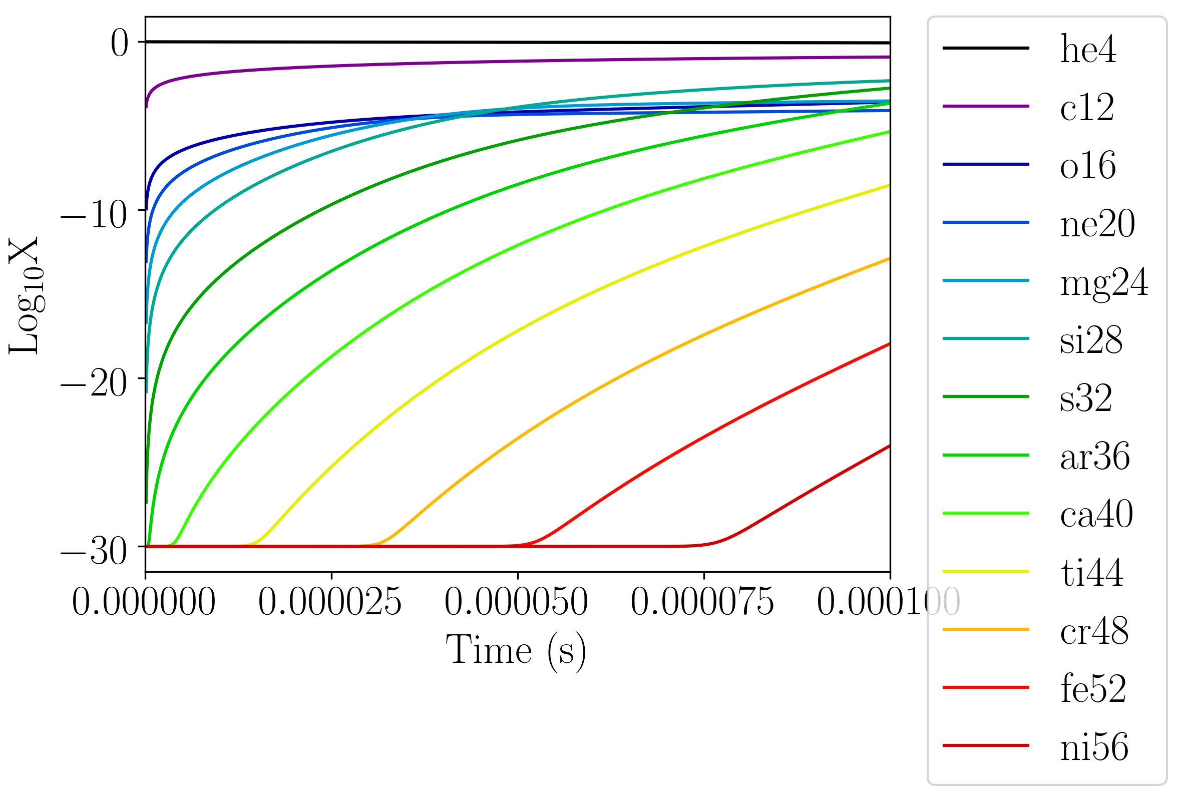
Fig. 1 An example of a plot output by the burn_cell unit test. This is the logX output corresponding to the network aprox13.
The file run-prefix_ydot.png and run-prefix_ydot.eps will display the
molar fraction (mass fraction / atomic weight) as a function of time,
both on logarithmic scales, for all species involved in the code.
The file run-prefix_T-edot.png and run-prefix_T-edot.eps will display
the temperature and the energy generation rate as a function of time.